Moments

Readings:

Ross: Chapter 2.4 & 2.5

Emile-Geay: Chapter 3

import numpy as np
import matplotlib.pyplot as plt
from scipy import stats

# These are some parameters to make figures nice (and big)
plt.rcParams['figure.figsize'] = 16,8
params = {'legend.fontsize': 'x-large',
          'figure.figsize': (15, 5),
         'axes.labelsize': 'x-large',
         'axes.titlesize':'x-large',
         'xtick.labelsize':'x-large',
         'ytick.labelsize':'x-large'}
plt.rcParams.update(params)

The n’th moment of a distribution is defined as as

\[ m(X,n)=E(X^n)=\sum_{i=1}^N x_i^nP(X=x_i)\]

\[ m(X,n)=E(X^n)=\int_\mathbb{R}x^n f(x)dx\]

for, respectively, discrete and continuous r.v.s. We will mostly be interested in the first two centered moments.

Expected value/mean

The expected value of a random variable is the average value we would expect to get if we could sample a random variable an infinite number of times. It represents a average of all the possible outcomes, weighted by how probably they are.

The expected value of a random variable is also called its first order moment, mean, or average. It is computed using the expectation operator:

\[\begin{split}E(X)=\mu=\begin{cases} \sum_{i=1}^{N}x_{i}P(X=x_{i}) & \text{if }X\text{ is discrete}\\ \int_{\mathbb{R}}x f(x)dx & \text{if }X\text{ is continuous} \end{cases}\end{split}\]

The expected value is also sometimes denoted using the bracket notation. We will make use of this later on:

\[\left < X\right> = E(X)\]

Examples

Bernoulli random variable. For a binomial random variable \(X_{bin}\) with \(p=0.5\), the possible outcomes are 0 and 1, and the probabiltiy mass function (pmf) is given by \(p(0)=p(1)=0.5\). In this case, the Expected value, or mean, is

\[ E(X)=\left<X\right> = \sum_{i=1}^{2}x_{i}P(X=x_{i}) = 0\cdot P(X=0) + 1 \cdot P(X=1) = 0\cdot 0.5 + 1\cdot 0.5 = 0.5\]

since \(p(X=x_i)=1/6\) for \(x_i\in \{1,\ldots,6\}\):

\[ E(X)=\left<X\right> = \sum_{i=1}^{6}x_{i}P(X=x_{i}) =\]

\[ = 1\cdot 1/6+2\cdot 1/6+3\cdot 1/6+4\cdot 1/6+5\cdot 1/6+6\cdot 1/6=7/2=3.5\]

Continuous uniform random variable. Let’s now look at the continuous case, focusing first on a random variable that is uniformly uniform distribution over the interval \([a,b]\). the probability is \(f(x)=1/[b-a]\) if \(x\in[a,b]\) and \(0\) otherwise. So the expectation will be:

\[\int_{\mathbb{R}}xf(x)dx=\int_{a}^{b}x\frac{1}{b-a}dx=\left.\frac{1}{b-a}\frac{x^{2}}{2}\right|_{a}^{b}=\frac{1}{2}\frac{b^{2}-a^{2}}{b-a}=\frac{1}{2}\frac{(b+a)(b-a)}{b-a}=\frac{a+b}{2}\]

Gaussian random variable For a Gaussian/Normal random variable with pdf \(f(x)=\frac{1}{\sqrt{2\pi}\sigma}e^{\frac{1}{2}\left(\frac{x-\mu}{\sigma}\right)^{2}}\) it can be shown (Example 2.22 in Ross) that \(E(X)=\mu\). So the distribution of a gaussian random variable is itself written in terms of the the first moment \(\mu\).

Important

Key property of expectation: linearity

\[E(aX+bY)=aE(x)+bE(y)\]

where \(X,Y\) are random variables and \(a,b\) are constants.

We can also define the expected value, or mean, of any function of a random variable:

\[\begin{split}E(g(X))=\begin{cases} \sum_{i=1}^{N}g(x_{i})P(X=x_{i}) & \text{if }X\text{ is discrete}\\ \int_{\mathbb{R}}g(x)f(x)dx & \text{if }X\text{ is continuous} \end{cases}\end{split}\]

Exercise

Discrete uniform random variable (fair die). Check for yourself that the average roll of the fair dice, i.e. the expectation of discrete uniform random variable taking values between 1 and 6 is \(E(X)=3.5\).

---

Variance and Standard Deviation

A closely related notion to the second order moment is the variance or centered second moment, defined as:

\[V(X)=E([X-E(x)]^2)=E([X-\mu]^2)=\int_\mathbb{R}(x-\mu)^2f(x)dx\]

Expanding the square and using the linearity of the expectation operator, we can show that the variance can also be written as:

\[V(X)=E(X^2)-(E(X))^2=E(X^2)-\mu^2\]

or

\[ V(X)=\left< X^2 \right>-\left<X\right>^2 \]

Variance is often denoted by \(\sigma^2\), i.e. \(V(x)=\sigma^2_X\)

Derivation:The property above is important, and a useful case-study to exemplify the linearity property of the expectation operator. Let’s show that two ways of writing the variance are equivalent:

\[E([X-E(x)]^2)=E([X-\mu]^2)=E(X^2-2X\mu + \mu^2)=E(X^2)-2E(X\mu)+E(\mu^2)\]

Where we have used the linearity property. Now, if we keep in mind that while \(X\) is a random variable \(\mu=E(x)\) is a constant number, we can apply the linearity property to say that \(E(\mu X)=\mu E(x)=\mu^2\). Also, since \(\mu\) is just a number, \(E(\mu)=\mu\), and thus \(E(\mu^2)=\mu^2\). Thus,

\[E(X^2)-2E(X\mu)+E(\mu^2)=E(X^2)-2\mu^2+\mu^2=E(X^2)-\mu^2\]

*Standard deviation Another closely related measure is standard deviation, defined simply as the square root of the variance

\[\text{std}=\sqrt{V(X)}=\sqrt{E([X-\mu]^2)}\]

Variance and standard deviation are measures of the spread of a distribution.

Important

Key Properties of Variance

\[ V(X+b)=V(x)\]

\[ V(aX)=a^2V(x)\]

\[ \text{std}(aX)=a \cdot\text{std}(X)\]

Examples

Discrete uniform random variable (fair die). How do we find the variance and standard deviation of the outcome of a roll of the fair dice? Answer:

\[V(x)=E[X^{2}]-E[X]^{2}=\sum_{x=1}^{6}x^{2}P(X=x)-3.5^2\]

\[==1^{2}\frac{1}{6}+2^{2}\frac{1}{6}+3^{2}\frac{1}{6}+4^{2}\frac{1}{6}+5^{2}\frac{1}{6}+6^{2}\frac{1}{6}-3.5^2=\frac{91}{6}-3.5^2=2.92\]

Gaussian distribution The pdf of a normally distributed r.v. with location parameter \(\mu\) and scale parameter \(\sigma\) is

\[f(x)=\frac{1}{\sqrt{2\pi\sigma^2}}\exp\left[-\frac{1}{2}\left(\frac{x-\mu}{\sigma}\right)^2\right]\]

It can be shown (E.g. Ross Section 2.4, example 2.26) that

\[ V(X)=\sigma^2\]

\[\text{std}=\sigma\]

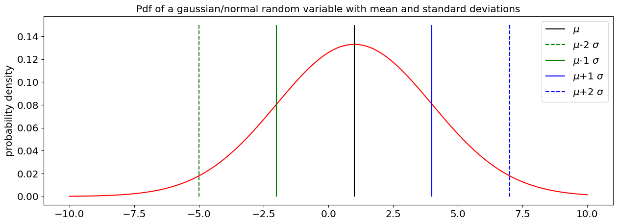
For a gaussian/normal random variable it’s worth remembering the 68-99-99.7 rule. That is, 68% of the values/outcomes of a gaussian/normal random variable lie within 1 standard deviation of th mean, 95% of the values lie within two standard deviations and 99.7% of the values lie within three standard deviations of the mean.

# let's plot the pdf of a gaussian random variable along with the standard deviation. 
# let's choose a gaussian/normal r.v. with mean(location) =1 and standard deviation (scale) =3

# define a vector of point at which to evaluate  the pdf 
mu=1;
sigma=3;
xlim_left=-10;
xlim_right=10;
x_norm=x_norm=np.linspace(xlim_left,xlim_right,1000)
pdf_norm=stats.norm.pdf(x_norm,loc=mu, scale=sigma)

fig, ax = plt.subplots(1)
plt.plot(x_norm,pdf_norm,'r')
plt.vlines(mu,0,0.15,label=r'$\mu$',color='k')
plt.vlines(mu-2*sigma,0,0.15,label=r'$\mu$-2 $\sigma$',color='g',linestyle='--')
plt.vlines(mu-sigma,0,0.15,label=r'$\mu$-1 $\sigma$',color='g')
plt.vlines(mu+sigma,0,0.15,label=r'$\mu$+1 $\sigma$',color='b')
plt.vlines(mu+2*sigma,0,0.15,label=r'$\mu$+2 $\sigma$',color='b',linestyle='--')
plt.legend()
plt.ylabel('probability density')
plt.title('Pdf of a gaussian/normal random variable with mean and standard deviations')

Text(0.5, 1.0, 'Pdf of a gaussian/normal random variable with mean and standard deviations')

Exercises

1. Continuous Uniform distributions The pdf of a r.v. uniformly distributed over the interval \([a,b]\) is \(f(x)=\frac{1}{b-a}\)

Show that

\[ V(X)=\frac{1}{12}(b-a)^2\]

2.Plot the pdf of a gamma distribution. Plto the pdf of a gamma distribution, along with its mean and standard deviations , specifically the points in the pdf that are, respectively, 1 and 2 standard deviations away from the mean. Choose shape parameter a\(=\alpha=3\) and scale parameter scale \(=\theta=1\). Use the scipy.stats.gamma method (documentation link ). You’ll need to know (e.g. Wikipedia) that for a gamma random variable \(\mu=E(X)=\alpha\theta\) and \(\sigma=\sqrt{V(X)}=\sqrt{\alpha\theta^2}\). Notice that the probability of an outocome that is two standard deviations lower than the mean is nil, while it is possible to get an outcome that is two standard deviations higher than the mean.

# Exercise Block

---

Covariance, Correlation

In practice we are often interested in more than one quantity. We could have more than one measurements, or more than one quantity we are trying to infer, or perhaps our model has more than one parameter. We thus need to be able to make statistical statements about more than one random variable at a time.

We have defined joint probability of two random variables as \(p(x,y)=P(X=x \text{ AND } Y=y)\) for discrete random variables and \(p(x,y)=P(X\in [x,x+dx{] \text{ AND }Y\in [y,y+dy])}\) for continuous random variables.

Expectations of multiple variables

Just like for a single random variable, we can define the expectation of a function of more than one random variable

\[\begin{split}E(g(X,Y))=\begin{cases} \sum_{i=1}^{N}g(x_{i},y_i)P(X=x_{i},Y=y_i) & \text{if }X,Y\text{ are discrete}\\ \int_{\mathbb{R^2}}g(x,y)p(x,y)dxdy & \text{if }X,Y\text{ are continuous} \end{cases}\end{split}\]

Sum and linearity

For this example, we’ll restrict ourselves to the continuous case. If g(X,Y)=X+Y, then

\[E(X+Y)=\int_{R^{2}}(x+y)p(x,y)dxdy=\int xp(x,y)dxdy+\int yp(x,y)dxdy\]

If we set \(g(x,y)=x\) and \(g(x,y)=y\) i the definition of expectation above, we can see that the first integral is just \(E(X)\) and the second integral is \(E(Y)\), so we recover the linearity property \(E(X+Y)=E(X)+E(Y)\).

Product and independence

Let’s now set \(g(X,Y)=XY\), then \(E(XY)=\int_{R^{2}}xy\cdot p(x,y)\cdot dxdy\). IF X and Y are independent, then \(p(x,y)=p(x)p(y)\) and some simple manipulation of the integral gives us \(E(XY)=E(X)E(Y)\). However, this ONLY holds IF the variables are independent. A very common mistake is to assume that the expectation of the product is equal tot he product of the expectations. This is not generally true.

Covariance

For variables that are not independent, we are often interested in how they relate to each other. The most common metric for that relationship is the covariance. We can define Covariance in a way that is analogous to variance:

\[ Cov(X,Y)=E[(X-E[X])(Y-E[Y])] =\left<\left(X-\left<X\right>\right)\left(Y-\left<Y\right>\right)\right>.\]

Note that if the means are zero, then \(Cov(X,Y)=E(XY)=\left<XY\right>\). Taking out the means just centers the random variables.

Similarly as for variance, we can use the linearity property of expectation to show that

\[ Cov(X,Y)=E[XY]-E[X]E[Y]=\left<XY\right> - \left<X\right>\left<Y\right>\]

\(Cov(X,Y)\) is also sometimes denoted as cross-covariance, while \(Cov(X,X)\) is called auto-covariance.

Important

Key Properties of Covariance

\[ Cov(X,Y)=Cov(Y,x)\]

\[ Cov(aX,Y)=a\cdot Cov(X,y)\]

\[ Cov(X,Y+Z)=Cov(X,Y)+COV(Y,Z)\]

\[ Var(X+Y)=Var(X)+Var(Y)+2Cov(X,Y)\]

Correlation

It is often practical to rescale the random variables and rescale the covariance to be between zero and one. One of the advantages of this rescaling is that it removes the dependence of X and Y on units.

The correlation coefficient is defined as:

\[ \rho=\frac{Cov(X,Y)}{\sigma_X\sigma_Y}\]

where \(\sigma_X=std(X)=\sqrt{Var(X)}\) is the standard deviation of X. The correlation coefficient always lies between -1 and 1. If \(0<\rho<1\) we would say the variables are correlated, if \(-1<\rho<0\) we would say the variables are anti correlated, and if \(\rho=0\) we would say the variables are not correlated.

The square of the correlation coefficient \(\rho^2\) quantifies the amount of variance that is shared between variables \(X\) and \(Y\).

Important

Key Properties of Correlation

\[ -1<\rho<1\]

If \(|\rho|=1\) the variabels are linearly related, i.e. \(X\) can be written as \(X=aY+b\).

Covariance Matrix The general way of writing the covariance between multiple random variables \(X_i\) is by using a covariance matrix \(\Sigma\), defined as

\[\Sigma_{i,j}=Cov(X_i,X_j)\]

For the case of two variables, \(X,Y\), the covariance matrix takes the form:

\[\begin{split} \Sigma_{XY}=\left[\begin{array}{cc} Cov(X,X) & Cov(X,Y)\\ Cov(Y,X) & Var(Y,U) \end{array}\right]=\left[\begin{array}{cc} Var(X) & Cov(X,Y)\\ Cov(X,Y) & Var(Y) \end{array}\right]\end{split}\]

By the definition of covariance, the covariance matrix can also be written as:

\[\begin{split}\Sigma_{XY}=\left[\begin{array}{cc} \sigma_{X}^{2} & \rho\sigma_{X}\sigma_{Y}\\ \rho\sigma_{X}\sigma_{Y} & \sigma_{Y}^{2} \end{array}\right]\end{split}\]

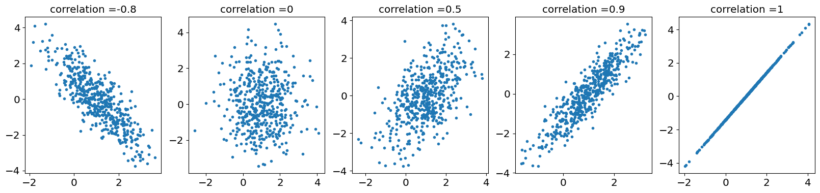
Example: Multivariate Normal

We’ll generate some draws from a multivariate normal distribution (Wikipedia link). This is a well-behaved joint distribution of normal/gaussian random variables. If two random variables are drawn from a bivariate multivariate normal, than both of them are normal, and they are correlated. The multivariate normal of dimension n is defined in terms of a vector of means containing the (marginal) means of each of those random variables, and a covariance matrix of size \(n\times n\) containing the variances and covariances between each set of random variables. We would denote this multivariate distribution by

\[ \mathbf{X}\sim\mathcal{N}\left(\mathbf{\mu,\Sigma}\right),\]

where \(\mathbf{X}=[X_1,X_2,\ldots,X_n]\) is a vector containing the correlated random variables \(X_i\).

We’ll draw some samples from a bivariate normal distribution below:

#parameters
rho_vals=[-0.8,0 , 0.5, 0.9 , 1]

fig,ax=plt.subplots(1,5,figsize=[20,4])
for j in range(5):
    mu_x=1     # mean of X
    mu_y=0     # mean of Y
    var_X=1    # Variance of X
    var_Y=2    # variance of Y
    rho=rho_vals[j]  # Correlation coefficient
    
    # make a covariance matrix
    mu_vec= np.array([mu_x,mu_y])
    cov_mat = np.array([[var_X, rho*np.sqrt(var_X*var_Y)], [rho*np.sqrt(var_X*var_Y), var_Y]])
    Xvec=stats.multivariate_normal.rvs(cov = cov_mat, mean = mu_vec,size=500)
    
    
    ax[j].plot(Xvec[:,0],Xvec[:,1],'.')
    ax[j].set_title('correlation ='+str(rho))

Exercise

Prove that \( Var(X+Y)=Var(X)+Var(Y)+2Cov(X,Y)\).

Hint Use \(Cov(X,Y+Z)=Cov(X,Y)+Cov(Y,Z)\) and \(Var(X)=Cov(X,X)\)

---

Correlation vs Independence

Note that while two independent random variables will have an correlation and covariance of 0, a correlation or covariance of 0 does not imply indepenence: Example

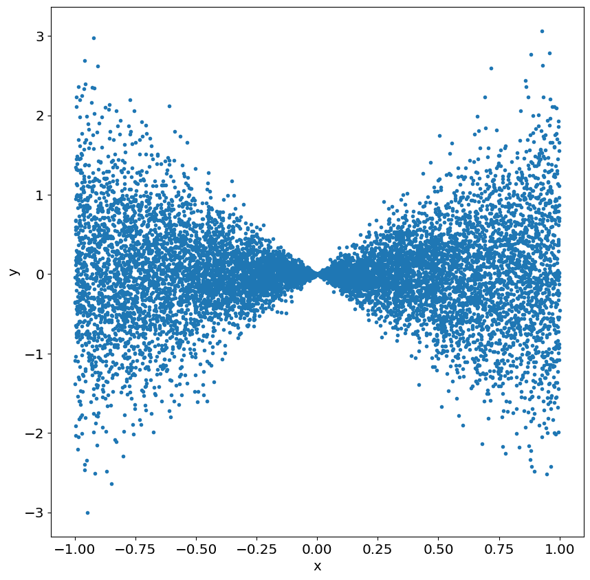
Example (in class):

We will go through this example in class

Consider two random variables, \(X\) and \(Y\). \(X\) is uniformly distributed over the interval \(\left[-1,1\right]\):

\[X\sim U[-1,1],\]

while \(Y\) is normally distributed (Gaussian), with a variance equal to \(X^{2}\). We would denote this as:

\[Y|X\sim\mathcal{N}\left(0,X^{2}\right),\]

to imply that

\[P(Y=y|X=x)=p(y|x)=\left(2\pi x^2\right)^{-1/2}\exp\left[-\frac{1}{2}\left(\frac{y}{x}\right)^2\right]\]

The two random variables are obviously not independent. Indepencene requires \(p(y|x)=p(y)\), which in turn would imply \(p(y)=p(y|x_1)p(y|x_2)\) for \(x_1\neq x_2\).

Prove analyitically and numerically that \(Cov(X,Y)=0\)
Hint: For the analytical proof, use the relation \(p(x,y)=p(y|x)p(x)\) to compute \(E(XY)\). Alternatively, you can use the same relation to first prove \(E(E(Y|X))\).

Analytical:

\[Cov(X,Y)=E(XY)-E(X)E(Y)=E(XY)\]

\[=\int_{-1}^{1}\int_{-\infty}^{\infty}x\cdot y\cdot p(x,y)\cdot dx\cdot dy=\int_{-1}^{1}\int_{-\infty}^{\infty}y\cdot x\cdot p(y|x)p(x)\cdot dx\cdot dy\]

\[=\int_{-1}^{1}\left[\int_{-\infty}^{\infty}y\cdot p(y|x)\cdot dy\right]x\cdot dx\]

\[=\int_{-1}^{1}\left[\int_{-\infty}^{\infty}y\cdot\frac{1}{\sqrt{2\pi x^{2}}}e^{-\frac{1}{2}\left(\frac{y}{x}\right)^{2}}\right]x\cdot dx\]

The inner integral is just the expected value of \(y\) for a constant \(x\), \(E(Y|X)\) and it is zero, since \(Y|X\sim\mathcal{N}\left(0,X^{2}\right)\). Thus, since the integrand is zero, the whole intergral is zero.

Ndraws=10000
X=stats.uniform.rvs(loc=-1,scale=2,size=Ndraws);
Y=np.zeros([Ndraws])
for i in range(Ndraws):
    Y[i]=stats.norm.rvs(loc=0,scale=np.abs(X[i]))

fig,ax=plt.subplots(1,figsize=[10,10])
plt.plot(X,Y,'.')
plt.xlabel('x')
plt.ylabel('y')

scov=1/(Ndraws-1)*np.sum((X-np.mean(X))*(Y-np.mean(Y)))

print(scov)

-0.0016495823691105975