2. The Hasselmann model

2. The Hasselmann model#

The Physical Basis: 1-Box model#

Consider the evolution of the energy budget of a linear system described by temperature \(T(t)\) , and forced by an external heat-flux \(F(t).\) Assuming the system has thermal inertia \(C\), we can write the general evolution of the model as:

\[ C\frac{dT}{dt}=Q\left(T\right)+F(t) \]

where \(Q(T)\) are heat fluxes that are caused as a response to temperature fluctuations.

Now consider a steady-state \(T_{0}\) with steady-state forcing \(F_{0}\), such that \(dT/dt=0\) and \(Q(T_{0})=F_{0}\). For small deviations in forcing \(\Delta F(t)=F(t)-F_{0}\) that lead to small deviations from steady state in temperature \(\Delta T(t)=T(t)-T_{0}\) such that \(\Delta T/T_{0}\ll1\). We can linearize the system thus:

\[ C\frac{dT}{dt}=Q\left(T_{0}\right)+\left.\frac{dQ}{dT}\right|_{T_{0}}\Delta T+\mathcal{O}\left(\left(\frac{\Delta T}{T_{0}}\right)^{2}\right)+F_{0}+\Delta F(t) \]

\[ C\frac{d\Delta T}{dt}=-\lambda\Delta T+\Delta F\left(t\right) \]

where \(\lambda\) is usually called the feedback. It can also be thought of as a restoring rate, or a damping rate. A larger value for \(\lambda\) means that an anomaly \(\Delta T\) will engender a larger negative heat flux -\(\lambda\Delta T\) that will tend to quickly damp the \(\Delta T\) anomaly. I’ve written \(\lambda=-dQ/dt\) because almost all the physical systems encountered in earth-sciences will have negative feedback. Having a positive feedback (\(dQ/dt>0)\) Implies the system is unstable and will blow up when taken out of its equilibrium point \(T_{0}.\) Thus, in our convention, \(\lambda\) will usually have positive values for a stable system. That being said, signs conventions vary wildly, and often times you will encounter \(\lambda=dQ/dt\) with \(\lambda\) taking negative values for a stable system.

The system will be characterized by two important parameters: (1) The first is the the equilibrium Sensitivity. At equilibrium:

\[ \frac{dT}{dt}=0\Rightarrow\frac{\Delta T}{\Delta F}=\frac{1}{\lambda}, \]

and (2) the characteristic time scale \(\tau_{0}\):

\[ \boxed{\tau_{0}=\frac{C}{\lambda}} \]

For the rest of the notes, we will drop the \(\Delta\) and assume that \(T,F\) and other variables represent small deviations from a steady state \(T_{0},F_{0}.\) The equation for the system can be written as

\[ \boxed{C\frac{dT(t)}{dt}=-\lambda T(t)+F\left(t\right)} \]

or, equivalently as:

\[ \boxed{\tau_{0}\frac{dT(t)}{dt}=-T(t)+\frac{1}{\lambda}F\left(t\right)} \]

This is just a simple 1-dimensional linear differential equation. The interesting part about it is that the forcing term \(F(t)\) is random. In the classic Hasselmann paradigm, \(F(t)\) is assumed to be uncorrelated white noise.

This type of box models are ubiquitous in Earth Sciences. The original Hasselmann model was used to represent variations in surface ocean temperatures, under the influece of heat exchanges with the atmosphere. The \(F(t)\) term represented weather anomalies which, on time-scales longer than the usual time-scale of weather phenomena (<2 weeks) could be considered to be random noise. In classical physics, this equation is called a Langevin equation or, in a slightly different form, an Ornstein-Uhlenbeck process.

Discretizing the Hasselmann model for simulations#

In this notebook we simulate some examples of the Hasselmann model and visualizing the spectrum. In order to simulate the above differential equation numerically, we have to discretize it. Taking a simple Forward-Euler finite difference scheme we can write:

\[ C\frac{T_{n}-T_{n-1}}{\Delta t}=-\lambda T_{n-1}+F_{n} \]

\[ T_{n}=\left(1-\frac{\Delta t\lambda}{C}\right)T_{n-1}+\frac{\Delta t}{C}F_{n}. \]

Denotinb

\[ \tau_{0}=\frac{C}{\lambda};\;\;\;\phi=1-\frac{\Delta t}{\tau_{0}};\;\;\;\varepsilon_{n}=\frac{\Delta t}{\tau_{o}}\frac{1}{\lambda}F_{n}; \]

the discrete version of the Hasselmann model thus becomes:

\[ T_{n}=\phi T_{n-1}+\varepsilon_{n} \]

Which is equivalent to an auto-regressive process of order 1, i.e. an AR(1) process.

The power spectrum#

Let’s simulate the Hasselmann model and visualize its spectrum.

Spectral estimators: to estimate the power spectra of a sample of \(F_n\) we will use the multitaper python package. Since our data are real, the spectra will be symmetric around 0, so we will generally only plot the positive frequencies.

To simulate the Hasselmann model we will need to choose some values of \(\tau_{0}\) and \(\lambda\) and decide on the variance \(\sigma_{F}^{2}\) of the white noise process \(F_{n}\). We will also need to choose a time-step \(\Delta t\) to discretize the differential equation.

White Noise#

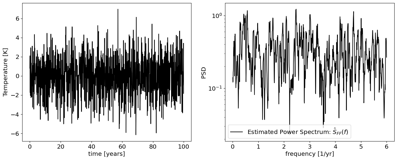
First, let’s visualize a white noise process, \(F_n\), which we’ll need in order to force the rest of the model.

# Set parameters
dt=1/12;     #time-scale. Let's say time is in years, and the time-step is 1 month, so 1/12 years.
T=100        # total integration time [years]
sigma_F=2    # variance of the forcing

# time-vector
t=np.arange(0,T,dt)
N=len(t)

#sample a gaussian white noise process (each F_n is independent and identically distributed, or i.i.d.).
F=stats.norm.rvs(loc=0,scale=sigma_F,size=N)


# Compute the spectral estimates
out=mtspec.MTSpec(F,nw=3,dt=dt,kspec=3)
f=out.freq       # freuencies
S_FF=out.spec    # power spectra
S_FF=S_FF[f>0]         # keep positive frequencies
f=f[f>0]

<matplotlib.legend.Legend at 0x135f47740>

../../_images/2772dfce9faf74cab84c36567c076778ae77e7eda15c33caec6e64c800c1f450.png

The power spectrum of a Hasselmann model#

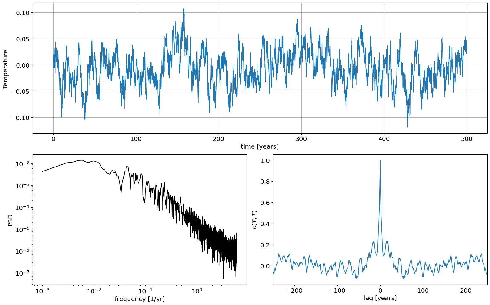
Now let’s simulate an actual Hasselmann Model.

You should play around and change the correlation time scale, \(\tau_0\), the forcing variance, and the feedback and see how the spetrum changes (you may need to keep note of the axis limits).

dt=1/12;     #time-scale. Let's say time is in years, and the time-step is 1 month, so 1/12 years.
T=500        # total integration time [years]
sigma_F=2    # variance of the forcing
tau_0= 3       # time-scale tau=C/lambda [years]
lam= 7       # feedback lambda

# time-vector
t=np.arange(0,T,dt)
N=len(t)

#sample a gaussian white noise process (each F_n is independent and identically distributed, or i.i.d.).
F=stats.norm.rvs(loc=0,scale=sigma_F,size=N)

# calculate phi and eps for the discretization
phi=   1-dt/tau_0
eps = (dt/tau_0/lam)*F;

## Simulate the Hasselmann model
#pre-allocate
T=np.zeros(N)

for n in range(1,N):
            T[n]=phi*T[n-1]+eps[n]

out=mtspec.MTSpec(T,nw=3,dt=dt,kspec=3)
f=out.freq
S_TT=out.spec
S_TT=S_TT[f>0]
f=f[f>0]

Let’s now plot the temperature time-series as well as the power spectrum and the autocorrelation function. We will use a log-log plot for the power spectrum.

../../_images/f6564d2f990322e96b9d9942a47fc9f001f1f81d7b569edc1d563cd469d120b0.png

Spectrum as a function of parameters#

The cell below plots time series, power spectra and auto-correlation functions for different values of the parameters.

Note that in the code below we prescribe the variance of the temperature time-series, rather than of the forcing.

Show code cell source Hide code cell source

#Discrete time series
dt=1/12;
T=500

sigma_vec=[1,3,9];
tau_vec=[0,0.7,15];

# Time Domain
t=np.arange(0,T,dt)
N=len(t)


plt.subplots(4,6,figsize=[16,12])
for ind_sigma in range(3):
    for ind_tau in range(3):
        # autocorrelation coefficient & total variance of the AR(1) process
        tau_0=tau_vec[ind_tau]
        sigma_T=sigma_vec[ind_sigma];
        
        if ind_tau==0:
            phi=0;
        else:
            phi=1-dt/tau_0
        
        #pre-allocate T
        T=np.zeros(N)

        ## Simulate AR1 process: note that the variance of the noise doesn't matter nowo, since we will rescale X)
        eps=stats.norm.rvs(loc=0,scale=1,size=N);
        for j in range(1,N):
            T[j]=phi*T[j-1]+stats.norm.rvs(loc=0,scale=1);
        
        #rescale X to have a given variance
        T=T*sigma_T/np.std(T)



        out=mtspec.MTSpec(T,nw=3,dt=dt,kspec=3)
        f=out.freq
        S_TT=out.spec
        S_TT=S_TT[f>0]
        f=f[f>0]

        acf=np.correlate(T,T,mode='full')
        acf=acf/np.max(acf)
        lags=np.arange(-N+1,N)
        
        ## Make Plots
    
        subplot_ind=6*(ind_sigma)+(ind_tau+1)
        plt.subplot(4,6,subplot_ind)
    
        plt.plot(t,T,'-')
        #plt.hlines(0,0,N,'r')
        plt.grid()
        plt.ylim(-20,20)
        plt.title(r'$\tau_0=$'+str(round(tau_0,2))+r'; $\sigma^2_T=$'+str(round(sigma_vec[ind_sigma])))
        plt.xlabel('j')
        plt.xlim(0,100)
        if ind_tau==0:
            plt.ylabel('y')

        subplot_ind=6*(ind_sigma)+3+(ind_tau+1)
        plt.subplot(4,6,subplot_ind)
        plt.plot(f,S_TT,'k',label=r'Estimated Power Spectrum: $\hat S_{FF}(f)$')
        #plt.hlines(sigma_eps**2*dt,np.min(f),np.max(f),'r',label=r'Theoretical Power Spectrum: $S_{FF}=$constant')
        plt.title(r'$\tau_0=$'+str(round(tau_0,2))+r'; $\sigma^2_T=$'+str(round(sigma_vec[ind_sigma])))
        
        plt.xscale('log')
        plt.yscale('log')
        plt.xlabel('frequency [1/yr]')
        plt.ylabel('PSD')
        plt.ylim(1E-3,1E3)
                

    
        plt.subplot(4,6,18+ind_tau+1)
        plt.plot(lags/12,acf,'-')
        plt.plot(lags/12,phi**(np.abs(lags)),'k',linewidth=3)
        plt.grid()
        plt.ylabel(r'$\rho(lag)$')
        plt.xlabel('lag [years]')
        plt.xlim(-20,20)


        plt.subplot(4,6,18+3+ind_tau+1)
        plt.plot(lags/12,acf,'-')
        plt.plot(lags/12,phi**(np.abs(lags)),'k',linewidth=3)
        plt.grid()
        plt.ylabel(r'$\rho(lag)$')
        plt.xlabel('lag [yrs]')
        plt.xlim(-20,20)
plt.tight_layout()

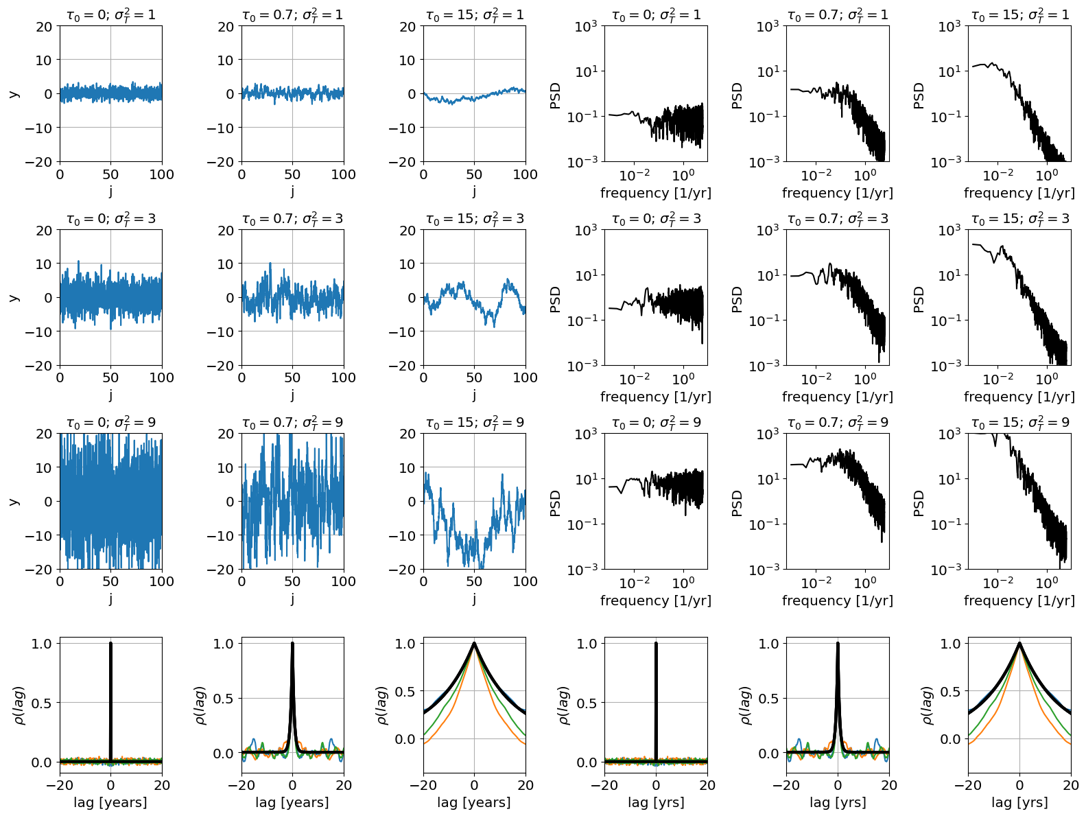
../../_images/b290caf71109079112641d836844952af4e47f4a4e6f76f9429be193731edd30.png

Note that the higher the time-scale \(\tau_0\), the more correlate the data. Indeed, \(\tau_0\) is the decorrelation time-scale. For the Hasselmann model, the expected correlation (black line) is \(\rho(T(t),T(t+\tau))=\exp^{-\tau/\tau_0}\). At the same time, \(1/\tau_0\) is also the frequency at which the power spectra goes from having a slope to being flat (i.e. “white”).

In general, the higher the average spectrum the more variance the time series. By the Parseval theorem, the variance is the integral of the PSD. So for processes where the power spectra have more spectral density at lower frequencies (i.e. the case of large \(\tau_0\)) more of the variance comes from these lower frequencies.